Cell Sensing, Implementation in CPM Code

Overview

Cells in a group communicate with one another in order to sense a gradient. We use a minimal adaptive model based on local excitation and global inhibition (LEGI). The network looks like the following

\[\begin{align*} S &\rightarrow S+X \ \ \ \ \ \ \ \ X \rightarrow R \\ S &\rightarrow S+Y \ \ \ \ \ \ \ \ Y \ \dashv \ R \\ \end{align*}\]

\(S\) is the signaling molecule representing the EGF gradient, \(X\) is the local reporter, \(Y\) is the global reporter, and \(R\) is the downstream readout.

Reactions for a specific cell

\[s_k \xrightarrow{\kappa} s_k + x_k \ \ \ \ \ \ \ x_k \xrightarrow{\mu} \emptyset \\ s_k \xrightarrow{\kappa} s_k + y_k \ \ \ \ \ \ \ y_k \xrightarrow{\mu} \emptyset \\\] \[y_k \rightleftharpoons_{\gamma_{<k>,k}}^{\gamma_{k,<k>}} y_{<k>}\] \[R_k = x_k - y_k\]

\(s_k\) is the local number of signaling molecules near cell \(k\), \(x_k\) is the number of local reporter molecules in cell \(k\) and \(y_k\) is the number of global reporter molecules. As well as being produced by the signaling molecule, \(y_k\) can also be exchanged between its neighbors. \(<k>\) represents the set of all cells neighboring cell \(k\). The rate \(\gamma\) at which cells exchange \(y\) depends on the size of the cell-cell contact.

\(R_k\) is the difference between the local and global reporters. A positive value of \(R_k\) reinforces cell \(k\)’s polarity vector in the direction of motion whereas a negative \(R_k\) does the opposite.

Chemical Concentration and Signal

There is a space dependent chemical concentration field. The chemical concentration has a constant gradient.

\[E(x,y) = gx + g_0 \\ [E] = \text{molecules} / \text{area}\]

The average signal from the chemical concentration that cell \(k\) feels is given as \(\bar{s}_k\). Diffusion is Poissonian so the variance in the measured signal \(s_k\) is equal to the average \(\bar{s}_k\).

\[\bar{s}_k = \int_k dA \ E(x,y) \\ \sigma_{s_k}^2 = \bar{s}_k\]

In the code this will be implemented by sampling values of \(s_k\) from a Gaussian distribution with the variance equal to the mean. Found a function that does this here (in module ran_mod).

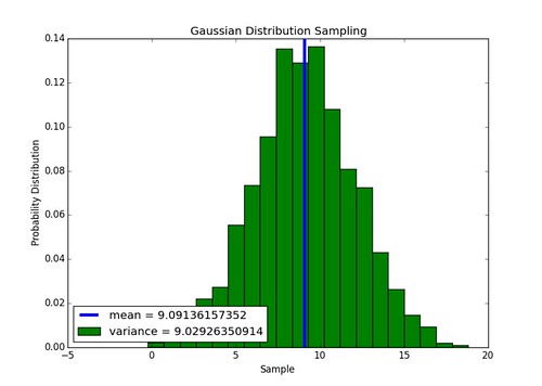
Implementation of Gaussian sampler works, above is an example of a 1000 numbers sampled from a distribution with a mean and variance of 9. The function is defined as normal(mean,sigma) in the module sensing.

We can place one cell in a chemical concentration with a linear gradient and see if sampling its measured signal yields a normal distribution of values.

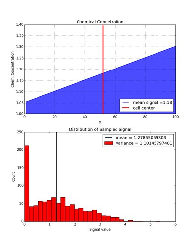
The distribution is not quite Gaussian anymore because values less than zero are not allowed. If the function getCellSignal( meanSignal) outputs a negative number then the signal value is set to zero. If this constraint is lifted, a Gaussian distribution is recovered.

Local Species

The local species \(x_k\) is the local reporter of the chemical signal that cell \(k\) measures. The dynamics of the local reporter satisfy the stochastic equation

\[\dot{x}_k = \kappa s_k - \mu x_k + \eta_{x_k} \\ \eta_{x_k} = \sqrt{\kappa\bar{s}_k}\xi_2 - \sqrt{\mu \bar{x}_k} \xi_3\]

\(\xi_i\) are unit Gaussian variables that make-up the noise \(\eta_{x_k}\) in the local reporter. In steady-state we can solve for \(x_k\) and \(\bar{x}_k\).

\[\bar{x}_k = \frac{\kappa}{\mu}\bar{s}_k \\ x_k = \frac{\kappa}{\mu}s_k + \frac{1}{\mu}\eta_{x_k}\]

Similar to the chemical concentration signal we can sample \(x_k\) from a distribution. This is implemented in the function getLocalX( meanSignal, signal). This function takes a sampled signal value \(s_k\) and then samples values for \(\xi_i\) in order to calculate \(x_k\).

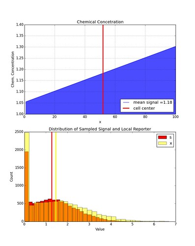
Here is an example of the distribution in values of \(x_k\) given some distribution of \(s_k\). Again, \(x_k\) is restricted to be non-negative values only.

Global Species

The global species \(y\) is the global reporter of the chemical concentration across all cells in the group. The number of the global species in cell \(k\) is given as \(y_k\). The dynamics of the global species is more complicated than the local one since it can diffuse to and from different cells.

\[\dot{y}_k = \kappa s_k - \mu y_k - y_k \sum_{<j,k>} \gamma_{j,k} + \sum_{<j,k>} y_j \ \gamma_{j,k} + \eta_{y_k}\]

The first two terms are the production and degradation rates of \(y_k\), same as in the case for \(x_k\). The first summation term accounts for the loss of \(y_k\) due to the movement of the global reporter into neighboring cells. The notation \(<j,k>\) represents all nearest neighbor pairs. Similarly, the second summation term accounts for the gain in global reporter moving into cell \(k\) from neighboring cells.

The movement of \(y\) in and out cells depends on the size of the boundary overlap between nearest neighbors and so \($\gamma_{<j,k>}\) must account for that. We choose that the magnitude of \(\gamma_{<j,k>}\) be proportional to the size of the boundary overlap.

\[\gamma_{<j,k>} = G L_{<j,k>} \\ L_{<j,k>} \equiv \text{Length of boundary overlap}\]

Note that \(\gamma_{j,k}\) has a few interesting properties.

\[\gamma_{j,k} = \gamma_{k,j} \ \ \ \ \ \ \ \gamma_{j,j} = 0\]

It is also useful to know the sum of all the contributing exchanges between cell \(k\) and all the other cells and define that to be \(\Gamma_k\).

\[\Gamma_k = \sum_{j=1}^N \gamma_{j,k}\] \[\Rightarrow \dot{y_k} = \kappa s_k - \mu y_k - \Gamma_k y_k + \sum_{j=1}^N y_j \ \gamma_{j,k} + \eta_{y_k}\]

The steady-state solution can be written in terms of vectors.

\[\kappa \vec{s} + \vec{\eta}_y = M \ \vec{y}\]

\(M\) is a square, symmetric matrix governing degradation and exchange of the global reporter in all cells.

\[M = \begin{bmatrix} \mu+\Gamma_1 & -\gamma_{1,2} & \cdots & -\gamma_{1,N} \\ -\gamma_{2,1} & \mu+\Gamma_2 & \cdots & -\gamma_{2,N} \\ \vdots & \vdots & \ddots & \vdots \\ -\gamma_{N,1} & -\gamma_{N,2} & \cdots & \mu+\Gamma_N \end{bmatrix}\] \[\begin{align*} \eta_{y_k}&= \sqrt{\kappa \bar{s}_k} \xi_4 - \sqrt{mu\bar{y}_k} \xi_5 - \sum_{j=1}^N\sqrt{\bar{y}_k \gamma_{j,k}} \ \chi_{j,k} + \sum_{j=1}^N\sqrt{\bar{y}_j \gamma_{j,k}} \ \chi_{j,k} \\ \eta_{y_k} &= \sqrt{\kappa \bar{s}_k} \xi_4 - \sqrt{mu\bar{y}_k} \xi_5 + \sum_{j=1}^N \left[ \chi_{j,k} \sqrt{\gamma_{j,k}} \left( \sqrt{\bar{y}_j}-\sqrt{\bar{y}_k} \right) \right] \end{align*}\]

As in the local species case, \(\xi_i\) and \(\chi_{j,k}\) are unit Gaussian variables that contribute to the noise in the global reporter. In order to compute \(\eta_{y_k}\) we need to know the average number \(\bar{y}\) in every cell.

\[\begin{align*} \kappa \vec{\bar{s}} &= M \ \vec{\bar{y}} \\ \Rightarrow \vec{\bar{y}} &= \kappa \ M^{-1} \ \vec{\bar{s}} \end{align*}\]

Using this we can then solve for the actual measured value of the global reporter in each cell \(\vec{y}\).

\[\vec{y} = M^{-1} \left( \kappa \vec{s} + \vec{\eta}_y \right)\]

Implementation

All possible values of \(\gamma_{j,k}\) are stored in an array gNN, such that gNN(j,k) corresponds to \(\gamma_{j,k}\). Below is a list of subroutines/functions that implement the above dynamics.

• Subroutine makeMtrxGamma( gNN, N, rSim, sigma, x) calculates all \(\gamma_{j,k}\) values.
• Subroutine makeMtrxM( gNN, M, N) calculates the values of all matrix elements \(M_{j,k}\).
• Subroutine getMeanY( meanSignal, M, meanY, N) calculates the vector \(\vec{\bar{y}}\).
• Subroutine getEtaY( etaY, gNN, meanSignal, meanY, N) calculates the vector \(\vec{\eta}_y\).
• Subroutine getSpeciesY( etaY, M, N, signal, y) calculates the population of \(y\) in each cell.

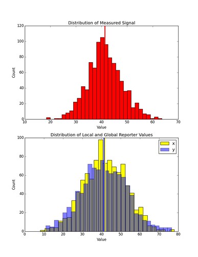
Here is an example of the distribution in values of \(x_k\) and \(y_k\) given some distribution of \(s_k\) in a simulation involving only one cell. The chemical concentration profile has the same gradient as in the previous examples, but the off-set has been increased.

Downstream Readout

Once the values of \(x_k\) and \(y_k\) are calculated for all cells involved we can measure the downstream output \(R_k\).

\[\vec{R} = \vec{x} - \vec{y}\]

Below is the result over many instances (1000) of a simulation involving a chain of 10 cells sitting parallel to the chemical gradient. Each data point represents the mean value of \(R\) at each cell, and the errors bars represent \(\pm\) one standard deviation.

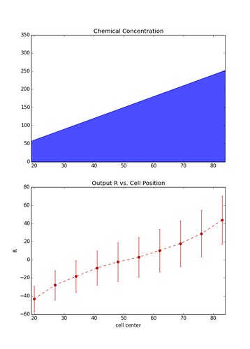
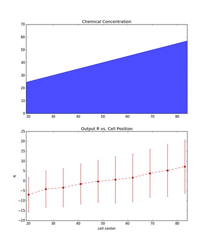
The figure on the left is representative of simulations with a relatively large gradient whereas the figure on the right is of simulations with a shallow gradient. As you can see the larger the gradient the less noisy the output becomes.

Polarization and Bias

The cell sensing and signaling network will influence the polarization of the individual cells which will in turn affect the bias term in the CPM simulations.

Polarization

It is the downstream output \(R_k\) which will contribute to the change in the cell’s polarization vector. The change in the polarization vector of cell \(k\) at every Monte Carlo time step is given as

\[\Delta\vec{p}_k = -r\vec{p}_k + \epsilon \tfrac{R_k}{R_0} \Delta\vec{x}_k \\ R_0 \equiv g \sqrt{NA_0^3}\]

\(R_0\) is the expected signaling molecule difference across the whole cluster of cells. The purpose in dividing by \(R_0\) is to attempt to normalize \(R_k\) so that \(\epsilon\) may be used as a tuning parameter on the order of 1 in order to vary the strength of cell-cell communication.

Bias

The bias is modified in order to eliminate the need for the parameter \(P\). With the above expression for \(\Delta\vec{p}_k\) the term

\[w = \sum_{k=\sigma(a),\sigma(b)} \frac{\Delta\vec{x}_{k(a \to b)} \cdot \vec{p}_k}{ |\Delta\vec{x}_{k(a \to b)}| |\Delta\vec{x}_{k(\Delta t)}|}\]

Issues with this Model of Polarization & Bias

This model produces unrealistic results. Although cells properly sense their environment, this does not translate into relatively quick, coherent motion in the direction of increasing signal concentration as desired. Even in the case of a steep gradient, cells do not behave as expected.

In this video each of the 6 cells is colored to indicate their \(R_k\) value. Hot colors represent large, positive values whereas cool color represent smaller/negative values. The chemical gradient increases linearly from left to right.

As you can see cell movement does not look coordinated and the polarization vectors change erratically. Cells are properly measuring and communicating the signal as indicated by the right-side of the group generally having the largest values for the downstream readout. This means that the problem in the model lies in translating the various values of \(R_k\) to the dynamics of each cell which is done through the polarization and the bias.

I believe that the problem is most likely caused by the calculation of the change in polarization. Say that a cell at the very right edge of the group has both \(\vec{p}_k\) and \(\Delta\vec{x}_k\) pointing perpendicular to the gradient then its positive readout \(R_k\) would only reinforce movement perpendicular to the gradient. Other problems also occur when a cell becomes disconnected form the group.

Updated Polarization Implementation

These problems stem from the fact that the influence of sensing on polarization occurs through scaling \(\Delta\vec{x}_k\). Whereas it should depend on where the cell is located in the group. I propose that changes in polarization obey the following equation

\[\Delta\vec{p}_k = -r\vec{p}_k + \Delta\vec{x}_k + \epsilon \tfrac{R_k}{R_0} \vec{q}_k \ .\] \[R_0 \equiv g \ (N_g-1) \sqrt{A_0^3} \\ N_g \equiv \text{Number of cells parallel to the gradient}\]

The vector \(\vec{q}_k\) points away from all cell \(k\)’s neighbors.

\[\vec{q}_k = \sum_{<j,k>} L_{<j,k>} \frac{\vec{x}_k - \vec{x}_j}{|\vec{x}_k - \vec{x}_j|}\]

Using this implementation of updating the polarization vector yeilds results which are much more in-line with expectations.

Here are two preliminary simulation videos.

Qualitatively, the behavior is good but parameters need fine-tuning in order to get cells of desired sizes/shapes. The chemical gradient increases linearly from left to right, and there is about a +100 increase in the chemical concentration initially, between the cells.

Julien Varennes

Written with StackEdit.