The Algorithm

There are three cases that the code handles.

1. Single cell diffusion
2. Edge cell diffusion
3. General case diffusion

The single cell case is treated as a simple random walk. The edge cases and the general case are the more involved scenarios. Since cells can stretch or compress there are many different scenarios that can take place when cells try to move. The method used to determine which possible outcome will be chosen is explained at the bottom of the page.

Edge Case

The edge case refers to the cell at the end or the beginning of the 1D chain of cells. Since this cell has only one neighbor this leads to different scenarios then the general case. In the following pictures assume that the yellow cell is the edge cell, and that the blue cell is its neighbor.

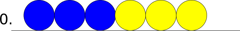
If the edge cell wants to move in – the leftward direction – there are the following possible states.

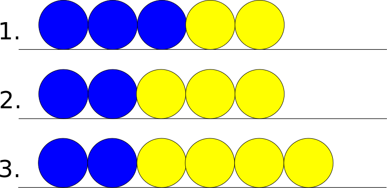
If the edge cell wants to move out – the rightward direction – there are the following possible states.

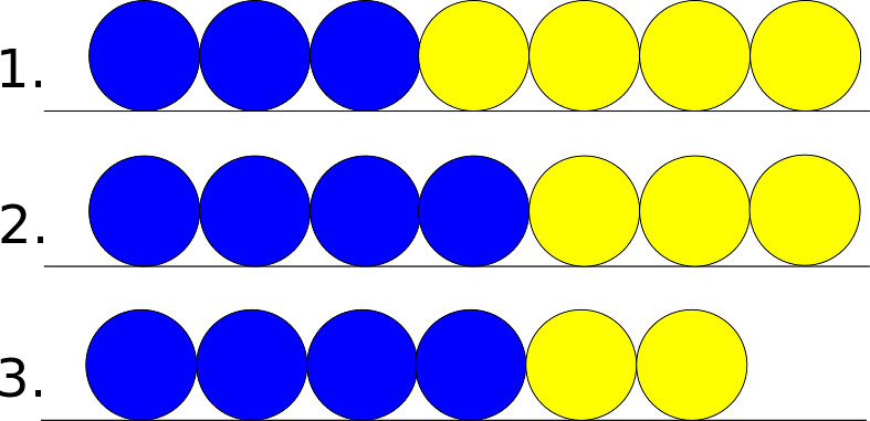
If the edge cell had been on the left as opposed to the right, the possible outcomes would be the reflections of the ones listed above.

General Case

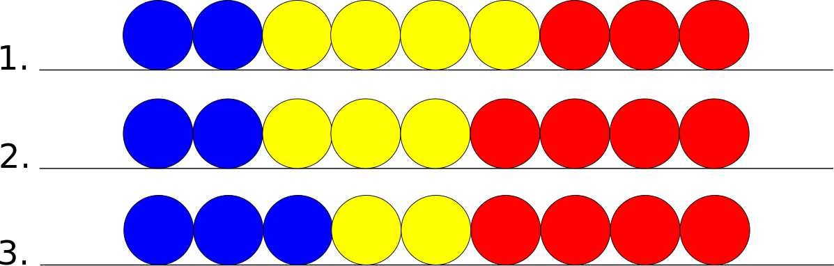
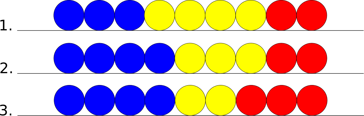
The general case refers to a cell in the middle of the chain. This cell has neighbors on both of its sides. In the following pictures assume that the yellow cell is the principal cell, the blue cell is its left neighbor, and the red cell is its right neighbor.

If the principal cell wants to move leftward there are the following possible states.

If the principal cell wants to move rightward there are the following possible states.

Choosing the State

We need a method to determine which state will be the chosen outcome. This is done by calculating the Hamiltonian of each state and then assigning a probability to that state. For a given state \(s\) the Hamiltonian is given by

\[H_s = \sum_{j=1}^N \lambda\left(V_j-V_0\right)^2 - f\Delta x \ .\\ \begin{align*} \lambda &\equiv \text{compression coefficient} \\ V_j &\equiv \text{volume off cell j} \\ V_0 &\equiv \text{relaxed cell volume} \\ f &\equiv \text{force cell exerts} \\ \Delta x &\equiv \text{cell displacement} \end{align*}\]

The sign of \(\Delta x\) depends on whether the cell’s center of mass moves to the left(-) or to the right(+). The direction of the force is chosen randomly at the beginning of each calculation. This will bias the principal cell’s movement either to the left or right.

\[f = \pm \vert\vec{f}\vert\]

The probability is given by

\[p_s \propto e^{-\beta H_s} \ .\]

The probabilities are normalized by summing over all the Boltzmann factors of the possible outcomes and the original state. The outcome is then chosen based on those normalized probabilities.

\[Z=\sum_s e^{-\beta H_s} \ \rightarrow \ p_s=\frac{e^{-\beta H_s}}{Z} \\ \beta\equiv\frac{1}{kT}\]

Simplifying parameters

We can simplify our simulation by grouping together a lot of these parameters in order to have the probabilities depend on the least number of parameters possible.

\[\begin{align*} \alpha &\equiv \beta\lambda V_0^2\\ \gamma &\equiv \beta \vert f\Delta x\vert \end{align*}\]

And so our expression for the Hamiltonian reduces to the following:

\[\beta H_s = \sum_{j=1}^N \alpha\left(\frac{V_j}{V_0}-1\right)^2 - \sigma_s\gamma \\ \sigma_s = \begin{cases} +1, & \text{if }\vec{f} \ \text{and} \ \Delta x\text{ are parallel} \\ -1, & \text{if }\vec{f} \ \text{and} \ \Delta x\text{ are antiparallel} \end{cases}\]

Now we can use this expression to calculate the probabilities of different states using the same procedure outlined above. Our parameter space now only consists of \(\alpha\) and \(\gamma\) which are both dimensionless quantities.